File:Surface normal illustration.png
Jump to navigation
Jump to search

Size of this preview: 556 × 600 pixels. Other resolutions: 222 × 240 pixels | 445 × 480 pixels | 712 × 768 pixels | 949 × 1,024 pixels | 1,379 × 1,488 pixels.
Original file (1,379 × 1,488 pixels, file size: 24 KB, MIME type: image/png)
| Description |
العربية: الناظم على سطح منحني في نقطة ما هو نفسه الناظم على مستوي مماس عند تلك النقطة.
Bosanski: Normala na površinu u tački je isto što i normala na tangentnu ravan te površine u toj istoj tački.
Čeština: Normála k ploše v bodě je shodná s normálou k rovině tečné k dané ploše ve stejném bodě.
Deutsch: Die Oberflächennormale in einem Punkt entspricht der Normalen der Tangentenebene, welche die Oberfläche in diesem Punkt berührt.
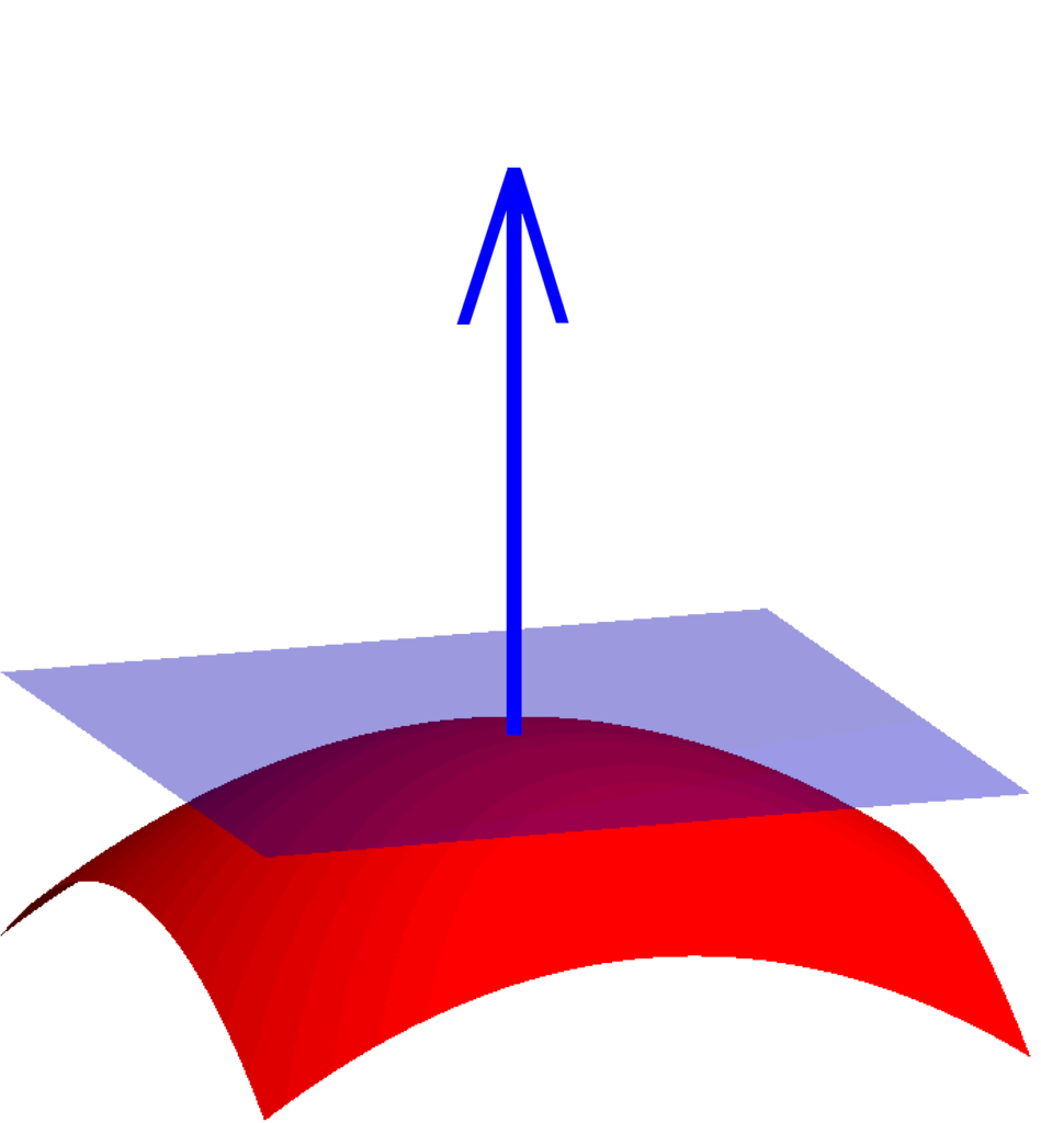
English: A normal to a surface at a point is the same as a normal to the tangent plane to that surface at that point.
Esperanto: Surfaca normalo kaj tanĝanta ebeno.
Hrvatski: Normala na površinu.
Italiano: Una normale ad una superficie è una normale al piano tangente nel punto.
Nederlands: De normaalvector van een 3D-oppervlak in een punt is de normaalvector van het raakvlak door dat punt aan het oppervlak door dat punt.
Polski: Konstrukcja wektora normalnego do powierzchni.
Svenska: Ytnormalen i en punkt på en slät yta är normalvektorn på tangentplanet till ytan i punkten.
ไทย: ค่านอร์มอลสำหรับจุดบนพื้นผิวหาได้จากค่านอร์มอลของระนาบสัมผัสที่สัมผัสพื้นผิวตรงจุดนั้น. |
|||
| Source | Own work | |||
| Author | Oleg Alexandrov | |||
| Other versions |
|


This diagram was created with MATLAB.
| I, the copyright holder of this work, release this work into the public domain. This applies worldwide. In some countries this may not be legally possible; if so: I grant anyone the right to use this work for any purpose, without any conditions, unless such conditions are required by law. |
Source code (MATLAB)
% an illustration of the surface normal

function main ()

% a few settings
   BoxSize=5;
   N=100;
   gridsize=BoxSize/N;
   lw=5;  % linewidth
   fs=35; % fontsize

% the function giving the surface and its gradient
   f=inline('10-(x.^2+y.^2)/15', 'x', 'y');
   fx=inline('-2*x/15', 'x', 'y');
   fy=inline('-2*y/15', 'x', 'y');

% calc the surface
   XX=-BoxSize:gridsize:BoxSize;
   YY=-BoxSize:gridsize:BoxSize;
   [X, Y]=meshgrid(XX, YY);
   Z=f(X, Y);

% plot the surface
   H=figure(1); clf; hold on; axis equal; axis off;
   view (-19, 14);
   surf(X, Y, Z, 'FaceColor','red', 'EdgeColor','none', ...
        'AmbientStrength', 0.3, 'SpecularStrength', 1, 'DiffuseStrength', 0.8);
   surf(X, Y, 0*Z+f(0, 0)+0.02, 'FaceColor', [0, 0, 1], 'EdgeColor','none', 'FaceAlpha', 0.4)

   camlight right; lighting phong; % make nice lightning

% the vector at the current point, as well as its tangent and normal components
   Z0=[0, 0, f(0, 0)];
   n=[fx(0, 0), fy(0, 0), 1];
   n=2*n/norm(n);

% graph the vectors
   HH=quiver3(Z0(1), Z0(2), Z0(3), n(1), n(2), n(3), 0.8); set(HH(1), 'linewidth', lw);

   set(HH(2), 'linewidth', lw)
   set(HH(2), 'XData', 0.4*[-0.78408 0 0.78408 NaN])
   set(HH(2), 'YData', 0.4*[0.78408 0 -0.78408 NaN])
   set(HH(2), 'ZData', 1*[14.824 17.2 14.824 NaN])

%  save to file
   print('-dpng',  '-r300', 'surface_normal_illustration.png');

%  This picture was tweaked in Gimp after being saved from MATLAB
%  to make the arrow look better.
File history
Click on a date/time to view the file as it appeared at that time.
| Date/Time | Thumbnail | Dimensions | User | Comment | |
|---|---|---|---|---|---|
| current | 03:31, 22 April 2007 | | 1,379 × 1,488 (24 KB) | wikimediacommons>Oleg Alexandrov | {{Information |Description= |Source= |Date= |Author= }} |
File usage
There are no pages that use this file.